Chapter 1 The empirical reference point of our model world

1.1 The national accounts

Among the official data collected by statistical institutes, the national accounts constitute the most important numerical record of overall economic activity. National accounts statistics are one of the most relevant empirical sources for macroeconomic discussions. Worldwide, the process of data collection is carried out by national and supranational statistical offices in accordance with some uniform rules. These rules are summarised in the UN’s System of National Accounts (SNA) and the European System of Accounts (ESA).¹

This chapter aims to develop an initial understanding of national accounts and of their key variables. The macroeconomic models that we will present in the following chapters have their empirical reference point in national accounts statistics. With these models, we attempt to establish and explain basic causal relationships between some important variables of the national accounts like gross domestic product, inflation and unemployment. A solid understanding of the main elements of national accounts is therefore of utmost importance for the understanding of what will follow in the book.

National accounts

National accounts are an “invention” of the 20th century but the first attempts to record macroeconomic activity can be dated back to the mid 18th century. A forerunner in this respect was the French economist and physician François Quesnay (1694-1774) who on behalf of the French monarchy started to develop a systematic approach to the study of economic activity. It was not until the tragic events of the Great Depression of the 1930s and of the Second World War that a systematic coverage of macroeconomic activity based on the circular flow representation of the economy put forward by John Maynard Keynes (1883-1946) finally emerged. From then on, national accounts were subject to continuous development and refinement. The improvement of national statistics was driven by the desire of policymakers to better assess the economic impact of their measures. Over the years, statistical frameworks have been repeatedly adapted and harmonised by international institutions like the United Nations and the European Union.

The annual brochures published by the Federal Statistical Office (Destatis) in Germany provide a good introductory overview and explanation of the German national accounts. See, e.g. Destatis (2021).

1.2 The circular flow of the macroeconomy

Before we begin with the study of the most important macroeconomic variables of the national accounts, we have to introduce some basic groups or sectors into which we can divide the economy. Once we have become familiar with these concepts, we will see how national accounts can be represented in circular flow type of relationship.

In the system of national accounts, the national economy is subdivided into sectors each of which perform a specific function:²

the corporate sector
the household sector
the government sector
the foreign sector

The corporate sector, the household sector together with the public, or government, sector, are the domestic sectors of the economy. Firms produce goods and services with the aim of earning a profit. A large part of national income, in the form of wages, capital or profit income, is generated in the corporate sector. This is also the sector undertaking most of the investment in the economy. The government sector, on the other hand, comprises those activities that are not guided by the profit motive and are independent of market dynamics. State, regional or local government firms are instead classified under the business enterprise sector if they produce goods and services for the market. Households, together with nonprofit private organisations (universities, labour unions, religious associations, etc.), form the household sector. This sector performs several functions. First of all, households consume the goods and services produced by the corporate sector. Second, households receive income from the corporate sector or from the government for providing factor services such as labour and capital that will be used in the production process. All economic activities that are not located on the national territory of the economy under consideration belong instead to the foreign sector.

To understand why we can represent the system of national accounts as a circular flow, we first look at a very simple example in which we include only two sectors, the corporate sector and the household sector. We will then expand our example by adding one by one the sectors that we have presented above. We will see how the economy can be represented as a closed system of accounts in which to every inflow corresponds an equal and offsetting outflow.

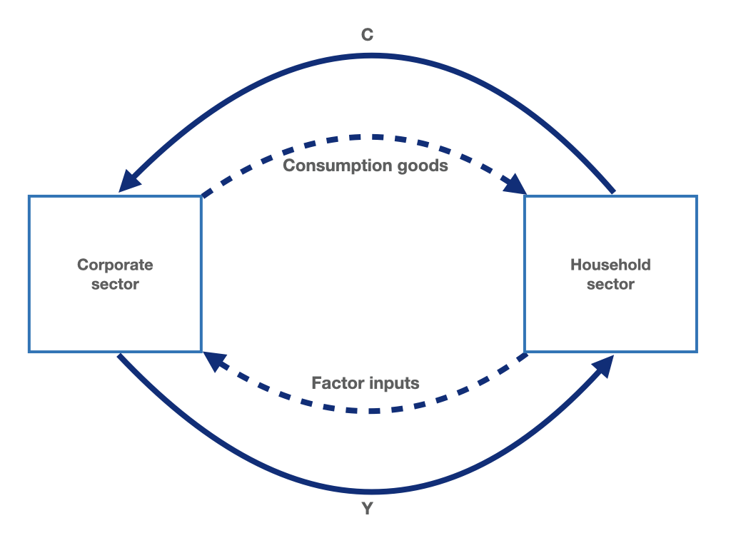
Figure 1.1: The simple macroeconomic circular flow with household and corporate sectors.

In figure 1.1, the dashed lines represent real goods and factor services while the solid lines represent the flow of payments. We observe how factor services (labour and capital) flow from the household sector to the corporate sector. At the same time, firms produce goods, e.g. consumer goods, which flow from the firm to the household sector. Consumption goods (\(C\)) produced by firms are bought by households out of the income (\(Y\)) they receive for providing firms with the necessary factors of production. Income received by households flows back to the firms in the form of consumption goods purchases. As we can see from figure 1.1, what is produced is consumed and nothing gets lost. The circular flow axiom applies:

\[\text{Sum of revenues} = \text{Sum of expenses}\]

We can start to extend our circular flow.³ We begin by assuming that households save part of their income.⁴ Saving (\(S\)) does not flow out of the circuit but it is absorbed, in accounting terms, into a new sector that we will call the capital formation sector. The circular flow axiom is still satisfied. As shown in figure 1.2, saving is matched by an equivalent amount that flows from the capital formation sector into the corporate sector. This quantity represents the investment (\(I\)) of the corporate sector.

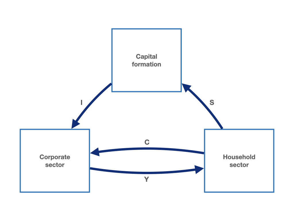
Figure 1.2: The macroeconomic circular flow with the household sector, the corporate sector and a capital formation sector.

The circular flow relationships can also be written using few equations. In equation (1.1), we see that household income (\(Y\)), flowing from the corporate sector to the household sector, equals the sum of consumption (\(C\)) and saving (\(S\)). Consumption and saving flow from the household sector to the corporate sector and the capital formation sector, respectively. At the same time, income (\(Y\)) is equal to the sum of consumption (\(C\)) and investment (\(I\)) represented with equation (1.2). It follows that in the capital formation sector, investment can only be equal to saving (equation (1.3)). The latter identity, i.e. equation (1.3), is to be understood as an ex-post identity, meaning that the equality between investment and saving is confirmed after the decisions about consumption and saving are made.

The circular flow in equations

\[\begin{equation} Y = C + S \tag{1.1} \end{equation}\]

\[\begin{equation} Y = C + I \tag{1.2} \end{equation}\]

\[\begin{equation} I = S: \text{ex post identity} \tag{1.3} \end{equation}\]

We can now increase the complexity of the circular flow by adding an additional element. We start by introducing the saving of the corporate sectors, the so-called retained earnings. In equation (1.4), total income (\(Y\)) is now composed of income of the household sector (\(Y_{h}\)) and saving of the corporate sector (\(S_b\)) (the arrows flowing out of the corporate sector in figure 1.3). At the same time, total income corresponds to the sum of household consumption expenditure (\(C_{h}\)) and firms investment expenditure (\(I\)), the arrows flowing into the corporate sector in figure 1.3. Income (\(Y_{h}\)) flows into the household sector and, as before, consumption (\(C_{h}\)) and saving (\(S_{h}\)) flows out of the household sector towards the corporate and the capital formation sector, respectively. In the capital formation sector, household saving and business saving (\(S_b\)) now add up to investment spending.

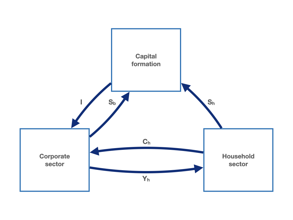
The macroeconomic circular flow with the household sector, the corporate sector, a capital formation sector and saving of the corporate sector.

Figure 1.3: The macroeconomic circular flow with the household sector, the corporate sector, a capital formation sector and saving of the corporate sector.

The following equation expresses the situation of figures 1.3:

\[\begin{equation} Y = Y_{h} + S_b = C_{h} + I \tag{1.4} \end{equation}\]

The circular axiom applies to each sector. In the corporate sector, we have that:

\[\begin{equation} Y_{h} + S_b = C_{h} + I \tag{1.5} \end{equation}\]

In the household sector, the following equation holds:

\[\begin{equation} Y_{h} = C_{h} + S_{h} \tag{1.6} \end{equation}\]

Finally, in the capital formation sector, we have that:

\[\begin{equation} I = S_{h} + S_b \tag{1.7} \end{equation}\]

We now introduce a fourth sector, the government. Just as before, households receives income from the corporate sector (\(Y_{h}^b\)). In addition, households receive now income from the government sector (\(Y_{h}^{g}\)). The income that households receive from the government can be for example labour or interest income that households receive as payments for the provision of their factor services. In addition, the household sector receives transfer payments (\(Tr\)) from the government. These may be pensions, unemployment benefits or other forms of support. The distinguishing feature of transfer payments is that they are received by households without anything in exchange.⁵ Additional revenues flow from the government to the corporate sector. These are subsidies (\(Z\)) and payments for the intermediate input of production (\(VL_{g}\)). Subsidies are provided by the state to the companies without any activity in exchange.⁶ The government pays companies for the purchase of intermediate goods and services that the government uses as intermediate production inputs for the undertaking of its own production of goods and services. At the same time, the government finances itself by collecting taxes from businesses (\(T_B\)) and households (\(T_{h}\)). These relationships are represented in figure 1.4 with the two arrows that flow into the government sector. We are not finished yet. The introduction of the government into the circular flow adds an additional element, which in figure 1.4 is represented by an additional arrow running from the government to the capital formation sector. This flow represent the saving of the government (\(S_{g}\)). The saving of the government can also be negative. In this case, the arrow would point in the opposite direction. The sum of government saving (\(S_{g}\)), household saving (\(S_{h}\)) and business saving (\(S_b\)) equals investment (\(I\)). Again, the circular flow axiom holds. The sum of revenues equals the sum of expenditures.

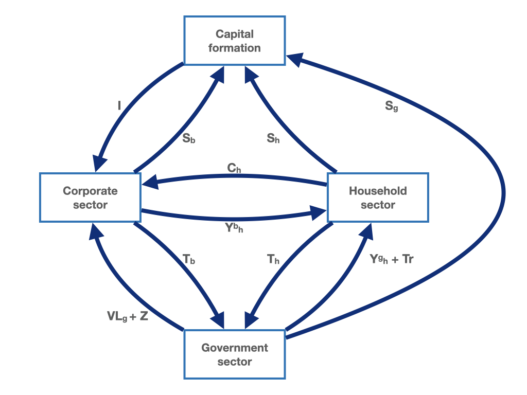
The macroeconomic circular flow with the household sector, the corporate sector, a capital formation sector, saving of the corporate sector and a government sector.

Figure 1.4: The macroeconomic circular flow with the household sector, the corporate sector, a capital formation sector, saving of the corporate sector and a government sector.

We can summarise our extended circular flow with the following set of equations:

Table 1.1: The macroeconomic circular flow.
	Income		Expenditures
Households:	\(Y_{h}^b + Y_{h}^{g} + Tr\)	=	\(T_{h} + C_{h} + S_{h}\)
Firms:	\(I + C_{h} + VL_{g} + Z\)	=	\(T_b + S_b + Y_{h}^b\)
Government:	\(T_{h} + T_b\)	=	\(Y_{h}^{g} + VL_{g} + Tr + Z + S_{g}\)
Capital formation:	\(S_{g} + S_{h} + S_b\)	=	\(I\)

We finally introduce the last element of our circular flow, the foreign sector. The last version of the circular flow including the foreign sector can be seen in figure 1.5. What is the role of the foreign sector in our circular flow? The foreign sector demands domestic goods and pays for domestic exports generating an additional source of revenue for domestic firms. In a specular manner, domestic firms pay for imports to the foreign sector. Exports and imports are indicated with the \(X\) and \(M\), respectively. The balance between the two flows may be positive or negative. If the domestic economy demands more than it sells to the foreign sector, i.e. it imports more than it exports (\(M - X > 0\)), a payment will flow from the foreign sector to the capital formation sector. In the long term, the foreign sector in part finances the domestic economy for the purchase of foreign goods. Conversely, if the exports of the domestic economy are larger than its import (\(M - X < 0\)), a payment will flow from the capital formation sector to the foreign sector. In the long term, the domestic economy in part finances the foreign sector for the purchase of domestic goods. The difference between exports and imports (\(X - M\)) is called the net exports or trade balance.

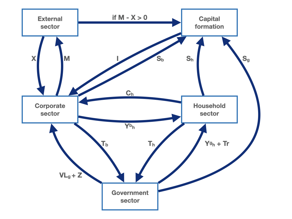
Figure 1.5: The macroeconomic circular flow with the household sector, the corporate sector, a capital formation sector and saving of the corporate sector, a government sector and theforeign sector.

In the capital formation sector, the sum of government, household and corporate saving equals the sum of investment and net exports. When net exports of the domestic economy are positive, i.e. when \(X - M > 0\), in the long run the domestic economy partly finances the purchase of domestic goods of the foreign sector. Conversely, when imports are greater than exports, in the long run foreign saving finances domestic demand. In equation form, we can summarise the capital formation sector as follows:

\[\begin{equation} S_{g} + S_{h} + S_b = I + (X - M) \tag{1.8} \end{equation}\]

We can now assume that the government mostly runs a budget deficit, i.e. has negative saving. We can rewrite equation (1.8) such that the sum of household saving (\(S_{h}\)) and business saving (\(S_b\)) equals the sum of investment (\(I\)), net exports (\(X - M\)), and government spending (\(G\)), where \(G = -S_{g}\):

\[\begin{equation} S_{h} + S_b = I + (X - M) + G \tag{1.9} \end{equation}\]

1.3 An important macroeconomic variable - GDP

One of the best known and most important macroeconomic variables in national accounts is Gross Domestic Product, or GDP for short. GDP represents a measure that attempts to capture the total production of an economy and the resulting income, the so called national income. As we can imagine, GDP is a key indicator of economic development. The total economic production is the quantity of goods and services produced in an economy in a given period of time, e.g., in a year. Likewise, national income is the income generated in an economy in a given period of time. The development of GDP is considered an important reference point for economic policy makers and economists. GDP, or aggregate output and national income, will be one of the central variables of the model economies that we are going to develop in the rest of this book.

A major challenge in calculating aggregate economic activity is the aggregation of a wide variety of goods and services into a single value. The goods and services produced in an economy differ in many ways, from the materials used, to the product characteristics and the production processes. How can we aggregate things as different as care in a kindergarten or nursing in a hospital with the programming work of artificial intelligence or the construction of a wind turbine into a single aggregate measure? To solve this problem, economists do not calculate GDP using quantities of goods and services (i.e. hours, pieces, kg, MB, KWh, etc.) but their value measured in monetary units such as the euro. This makes it possible to aggregate a wide variety of goods and services as their value is now expressed in a common monetary unit. But where do these values come from? For many goods and services, the value can be determined simply by looking at their market prices. However, for some goods and services observing the market price is simply not possible. Many goods and services are in fact not traded on the markets. Their value must be then estimated using other economic measures, such as production costs or by looking at the value of comparable goods.

Let us now try to imagine a simple economy in which only three goods are produced (1 year of childcare, 1 GB of artificial intelligence and a wind turbine), each with a value of €100. With a simple operation, we can now calculate the value of the gross domestic product of this very stylised economy.

\[\begin{gather} \text{GDP} = \nonumber \\ \text{1 year childcare} \cdot 100 \frac{€}{\text{year}} \nonumber \\ + \text{1 GB artificial intelligence} \cdot 100 \frac{€}{\text{GB}} \\ + \text{1 wind turbine} \cdot 100 \frac{€}{\text{piece}} \nonumber \\ = 300 € \nonumber \tag{1.10} \end{gather}\]

By denoting the units of goods and services produced with \(x_i\) and the prices per unit by \(p_i\), where the index \(i\) represents a particular good (e.g., \(x_1\) = good 1 and \(p_1\) = price of one unit of good 1), GDP is calculated as:

\[\begin{equation} BIP = x_1 \cdot p_1 + x_2 \cdot p_2 + x_3 \cdot p_3 = \sum_{i = 1}^{3}{x_i p_i} \tag{1.11} \end{equation}\]

The value of total economic activity in the eurozone, i.e., the sum of the values of all goods and services produced in the eurozone in 2019, “added up” to about 11.9 trillion euros, according to Eurostat (2020a), the statistical office of the European Union.⁷ In reality, the “addition” of the individual values is a more complex process. The simple summation that we have just seen is a strong theoretical simplification.

There are three different procedures or “approaches” for the calculation of GDP each of which correspond to one of the three definitions that are given to GDP. To calculate GDP we can look at the goods and services produced (production approach), the goods and services purchased (expenditure approach) and the income they generated (income approach). At theoretical level, the three different procedures and definitions must yield exactly the same numerical result. However, as with other empirical recording of a macroeconomic aggregates, statistical discrepancies often arise and values may differ depending on the procedure adopted. In the next subsection, we will introduce the three approaches for the calculation of GDP.⁸

1.3.1 Three definitions of GDP

Production

The first methodology to calculate GDP follows what is called the production approach. According to this methodology, GDP is calculated recording economic activity at the origin of production, i.e. the supply side of the economy. GDP is calculated summing the gross value added produced by firms, households and government. The gross value added is the production value of the goods and services produced by an economic entity minus the intermediate goods used in the production process that are purchased from an external supplier. The production value is measured initially at producer prices. These include all profits and costs incurred in production excluding indirect taxes net of subsidies.

With regard to the government as producer of goods and services, it is often the case that the government offers goods and services free of charge or just for a fee. In this case, only the costs of production are used. To arrive at GDP at market prices, indirect taxes must be added to the gross value added while subsidies must be subtracted. GDP at market prices is thus the value of all final products (not including intermediate inputs) produced within the geographic boundaries of an economy in a given period of time (e.g. in one year). GDP calculated with the production approach follows the so-called domestic concept or production location concept.

\[\begin{gather} \text{GDP}_{\text{at market prices}} \nonumber \\ = \nonumber \\ \text{Production of private firms}_{\text{at producer prices}} \nonumber \\ + \nonumber \\ \text{Production of households and private} \nonumber \\ \text{nonprofit organisations}_{\text{at producer prices}} \\ + \nonumber \\ \text{Government production}_{\text{at producer cost}} \nonumber \\ + \nonumber \\ \text{indirect taxes minus subsidies} \nonumber \tag{1.12} \end{gather}\]

Expenditure

The second definition and methodology for the calculation of GDP follows the expenditure approach. According to the expenditure approach, GDP is given by the sum of the expenditures on newly manufactured products within an economy produced in a given period of time. Expenditures may be for consumption purposes, investment activities, or demanded by the government. The only requirement is that the goods and services demanded are produced domestically. In addition to the purchase of goods and service by domestic entities, we must add the expenditures of foreign countries on domestic production and, at the same time, subtract the expenditures of the domestic entities on goods and services imported from abroad. This can be summarised as follows:

\[\begin{gather} \text{GDP}_{\text{at market prices}} \nonumber \\ = \nonumber \\ \text{Consumption expenditure of household} \nonumber \\ \text{and nonprofit institutions} \nonumber \\ + \nonumber \\ \text{Investment spending of businesses,} \nonumber \\ \text{government, households and} \nonumber \\ \text{nonprofit institutions} \\ + \nonumber \\ \text{Government consumption expenditure} \nonumber \\ + \nonumber \\ \text{Exports} \nonumber \\ - \nonumber \\ \text{Imports} \nonumber \tag{1.13} \end{gather}\]

The following table uses the expenditure approach and shows the values of consumption, investment, public demand, exports, imports and GDP for the euro area in the year 2019 using data from Eurostat (2020b).

Table 1.2: Nominal gross domestic product by expenditure approach, euro area, 2019. Source: Eurostat (2020b).
	Expenditures by category, current values, million euros
Final consumption expenditure of household and non-profit institutions	6378516.0
Government consumption expenditure	2456599.7
Gross investment	2741959.8
Net exports of goods and services	405647.8
Gross domestic product	11982723.3

Income

The third way to calculate GDP follows the so-called income approach. With this procedure, the Gross National Income is calculated (GNI for short). The GNI calculates the total sum of income earned within a period of time by all residents (nationals) of a country either through employment activities or capital ownership. The calculation of GNI makes no distinction whether the income is generated domestically or abroad (nationals concept = residence concept).⁹

If we subtract indirect taxes from GDP at market prices and add back subsidies, we arrive at GDP at factor costs. Factor costs are the costs associated with the factors of production (labour, capital, etc.), which in turn represent income received by those factors. Unlike GNI, GDP at factor cost captures the value of all income generated by productive activities within the boundaries of an economy (domestically) in a given period of time; i.e., regardless of whether it was generated by domestic or foreign residents (domestic concept = place-of-work concept).

The two main income categories in a capitalist economy are the wages of the production factor labour and the profits of the production factor capital. Wages include the actual gross wages of workers, the gross wages of employees as well as the employers’ contributions to social security. Profits consist of retained earnings of corporations, distributed profits (dividends), interest, rents and leases, and entrepreneurial income of the self-employed.

To arrive at the gross national income (of residents), the wage and profit income flowing to foreign countries must be subtracted from the GDP at factor cost, and the wage and profit income received by residents from abroad must be added. This is referred to as the primary income balance with foreign countries. As we said above, gross national income follows the nationals or residence concept. The following equations illustrate the calculation of GDP following the income approach:

\[\begin{gather} \text{GDP}_{\text{at market prices}} \nonumber \\ - \nonumber \\ \text{Indirect taxes} \nonumber \\ + \\ \text{Subsidies} \nonumber\\ = \nonumber \\ \text{GDP}_{\text{to factor income}} \nonumber \tag{1.14} \end{gather}\]

and:

\[\begin{gather} \text{GDP}_{\text{to factor income}} \nonumber \\ + \nonumber \\ \text{Inflow of primary income from abroad} \nonumber \\ - \nonumber \\ \text{Outflow of primary income to foreign countries} \nonumber \\ = \nonumber \\ \text{GNI} \\ = \nonumber \\ \text{Wage income}_{\text{of residents}} \nonumber \\ + \nonumber \\ \text{Profit income}_{\text{of residents}} \nonumber \tag{1.15} \end{gather}\]

The calculation of GDP according to the income approach requires the existence of data on corporate and property income. For some countries, including Germany, a stand-alone GDP calculation according to the income approach has not been possible so far due to the insufficient availability of data. The result is that data on corporate and property income are calculated as residuals.¹⁰

The equivalence of the three approaches

In the simplified case of a closed economy with no economic relationships with the rest of the world, the three definitions of GDP calculated using the production approach, the income approach and the expenditure approach must yield exactly the same result. Since in practice there are no economies completely closed to foreign exchange, this condition can be considered true only with respect to the world economy as a whole.

\[\begin{gather} \text{Total value of production} \nonumber \\ = \nonumber \\ \text{Total value of income} \\ = \nonumber \\ \text{Total value of expenses} \nonumber \tag{1.16} \end{gather}\]

The website of the Federal Statistical Office of Germany provides an illustration of the three definitions of GDP with data for Germany (Destatis 2020d).

1.3.2 GDP does not measure quality of life

GDP is a measure that was designed to capture overall market economic activity. For this reason, GDP should not be considered an indicator of population well-being or misinterpreted as a measure of quality of life.

For example, GDP does not provide direct information on the distribution of income among households. These considerations related to income distribution play an important role in the quality of life of the population. If an increase in GDP is accompanied only by an increase in the income of the richest 10% of households, this would hardly lead to an improvement in the quality of life of the entire population.

Another problem with the GDP indicator is that it does not measure those economic activities such as childcare and elderly care that take place within households and for which no income is generated but are of fundamental importance for the society. At the same time, there is a significant gender inequality in the burden of these activities as they are often carried out by women with potential negative effects on professional careers and income level. National accounts and GDP alone provide insights on none of these issues.

Another aspect of criticism is that economic activities of repair and reconstruction occurring after dramatic event such as traffic accidents, natural disasters, and other emergencies have a positive impact on the value of GDP. Increases in GDP are also associated with environmental damages and polluting activities. Not least, political stability and the population’s perception of security cannot be represented by national accounts.

For a comprehensive assessment of quality of life, various criteria relating to health, education, environmental conditions, security, the rule of law, family ties, social opportunities or opportunities for social participation, among other things, should be considered. Special indicators have been developed for this purpose. In particular, the attention on the appropriate recording of economic activity and quality of life has increased after the financial crisis of 2007/08.¹¹ One of the aims here is to develop alternative overall indicators, such as the Better Life Index of the OECD (2020) or the Human Development Index of the United Nations (2020).

1.4 Sectoral financial balances

In section 1.2, we have seen how the national accounts of an economy can be represented as a closed system of accounts, in which, by definition, the deficits of one sector must always be equal to the sum of the surpluses of the other sectors. With other words, if one sector has a deficit (in this case, we speak of a negative financial balance), all other sectors taken together must have a surplus vis-à-vis the deficit sector of exactly the same amount (a positive financial balance). This principles applies to the flows as well as to the resulting cumulative stocks. This means nothing more that the debt of one sector is always equal to the sum of the assets of the other sectors.

To illustrate this simple fact, we must first define the sectoral financial balances. To begin with, we distinguish between the private, the government and the foreign financial balance. We must first recall the circular flow axiom from section 1.2 and use it to define the financing balances of the respective sectors. Household saving (\(S_{h}\)) together with business saving (\(S_b\)) minus business investment (\(I\)) equal the financial balance, i.e., the surplus or deficit, of the private sector. We denote the financial balance of the private sector as \(FB_p\). We define government saving simply as government financial balance, \(FB_g\). When the government runs a deficit, we refer to it as negative government financial balance. When the government is in surplus, the government has a positive financial balance. We denote the financial balance of the foreign country by \(FB_f\). If the financial balance of the foreign country is positive, the foreign country exports more than it imports, i.e. the domestic country has a negative financial balance vis-à-vis the foreign country. In the opposite case, the domestic balance would be positive. The domestic financial balance is simply the net exports (or the current account) and corresponds to the negative of the financial balance of the rest of the world.

Table 1.3: Sectoral financial balances.
Financial balance of the private sector	\(FS_{p}\)	=	\(S_{h} + S_b - I\)
Financial balance of the government	\(FB_g\)	=	\(S_{g}\)
Financial balance of the foreign sector	\(FB_f\)	=	\(-(X - M)\)

Solving equation (1.8) from Section 1.2 to \(0\) and substituting the definitions of financial balances, we get:

\[\begin{equation} FB_p + FB_g + FB_f = 0 \tag{1.17} \end{equation}\]

In words, we have that:

\[\begin{gather} \text{Financial balance of the private sector} \nonumber \\ + \text{Financial balance of the government} \nonumber \\ + \text{Financial balance of the foreign sector} \nonumber \\ = \nonumber \\ 0 \nonumber \end{gather}\]

All sectoral balances resulting from the circular flow must add up to zero. This means that a balance is always equal to the negative of the sum of the other sectoral balances. If we are given two sectoral balances, we automatically know the third sectoral balance.

The usefulness and informative value of sectoral financial balances can be better illustrated with a practical example. Figure 1.6 shows the sectoral financial balances for Germany and Spain over the period from 1995 to 2018.

Figure 1.6: Sectoral financial balances for Germany and Spain. Source: AMECO (2020).

Let’s first look at the case of Germany. We see that the financial balance of the government in Germany (the blue line) was usually negative, meaning that the government was in deficit in most of the years. After the international economic crisis started in 2008, the government’s financial balance decreased significantly (to -4.2% in 2010). Since 2012, however, the government financial balance in Germany has been close to zero and sometimes even slightly positive. The balance of the private sector (households and corporations) has been positive in Germany, except in 2000. This is represented by the green line. Since from equation (1.17), we know that the financial balances of the private, the government and the foreign sector the must add up to zero, we can calculate the financial balance of the foreign sector. Let’s try this exercise for 2012. In 2012, the government sector had a roughly balanced budget of -0.03%, while the private sector had a positive balance of 7.11%. Given these values, we can very well expect that the balance of the foreign sector (the red line) in 2012 must be about -7.14% of GDP, which is exactly what we observe. We must not forget that this figure also represents Germany’s current account surplus vis-à-vis the rest of the world, a well-known fact.

A question arises at this point. Is the fact that Germany has such a high external surplus a good or a bad thing? By maintaining a positive current account balance with foreign countries since the beginning of the millennium, Germany has been steadily building up foreign assets. That sounds good at first. However, one problem is that if Germany builds surpluses, at least one other country or many other countries together must have a deficit vis-à-vis Germany, which exactly offsets the German surplus (remember the circular axiom). Thus, a sustained current account surplus can only be achieved if the rest of the world borrows continuously from the surplus country. Can this be economically sustainable?¹²

Let’s now look at the sectoral financial balances of Spain. Looking at figure 1.6, we see that the sectoral balances of the country form a mirror image of Germany with a current account deficit. From 2000 onward, the Spanish government (the blue line) recorded just small deficits with some surpluses immediately before the financial crisis of 2008. In 2007, however, the private sector was running a very large deficit reaching 11% of GDP (the green line). This large negative sectoral balance of the private sector had to be offset by government and foreign surpluses. The foreign surpluses are simply the combined domestic deficit, i.e. the Spanish current account deficit, vis-à-vis the rest of the world.

Due to the outbreak of the global financial crisis, the private sector in Spain was no longer able to take on more debt and from 2009 had to consolidate. This is the reason why the green line in figure 1.6 in the graph for Spain goes up rapidly from 2007 onwards and, at the same time, the government balance (the blue line) goes down. The rapid increase in the Spanish government’s deficit indicates that the government had to intervene in order to prevent the Spanish economy from declining even further. At the same time, the deficit of the country vis-à-vis the rest of the world (or the surpluses of the foreign sector) decreased significantly (the red line). The graph clearly shows how Spain gradually reduced its current account deficit starting from 2008. When a country builds up large deficits with the rest of the world, it is only a matter of time before the process of over-indebtedness becomes unsustainable. When international creditors begin to have doubts about a country’s solvency, a debt crisis can easily erupt. Persistent current account surpluses, as well as persistent current account deficits (we speak of “external imbalances”) are followed by unstable debt dynamics which eventually lead the country to adoption corrective measures often accompanied by additional economic problems.

The euro area crisis highlighted the imbalances that were building up since 1999 and the establishment of the European Monetary Union. In figure 1.7, we see how essentially almost only one country (Germany) has accounted for the entire current account surpluses of the euro area since the turn of the millennium.¹³ This contrasts with some large deficits registered by other countries. For a long time, these countries were Spain, Greece, Italy and, increasingly from 2005, France. In this respect, we can say that Germany’s surpluses were offset by the deficits of the other euro area members.

More recently, we can observe that the euro area as a whole started to accumulated large surpluses. In figure 1.7, surpluses and deficits in the euro area were roughly on balance until around 2008. From 2008 onward, however, the balance became rather a surplus, with the consequences that the instabilities that had building up in the euro area are now building up between the euro area and the rest of the world.

Figure 1.7: Current account balances in the euro area. Note: Click on a country name to hide the country from the graph. Source: AMECO (2020).

Finally, figure 1.8 shows the net international investment position for some selected countries of euro area starting in year 2000. The net international investment position represents a stock variable and is the result of the accumulation of the previous current account positions. Financial balances indicate in fact the change in the net international investment position of a country, which in turn can be seen as an indicator of debt, if negative, or of external assets, if positive. From figure 1.8 we see how, in the case of Germany, net external assets have been steadily increasing. In 2019, Germany’s net international investment position reached above 70% of GDP. For the Netherlands, the figure was close to 90%. This contrasts with the situation for some of the highly indebted countries of the euro area such as Greece, Ireland, Portugal and Spain and to a minor extent with the situation of France, Italy and Austria which have a smaller negative net international investment position.

Figure 1.8: Net international investment position in the euro area. Source: Eurostat (2020b).

1.5 Growth rates of economic variables

Discussions in the media about economic developments, as well as in the debate in economic policy circles, do not focus on the level (the amount) of GDP but rather on the change of GDP relative to a previous period, being it a year or a quarter. In this case, we speak of a growth rate and in this particular case of the growth rate of GDP. The same is true for the price level, which is often reported as the percentage change with respect to the previous period, a measure commonly known as the inflation rate. The growth rate of a variable \(X\) expressed in percentage terms can be calculated using the following simple formula:

\[\begin{equation} \text{Growth rate of X in percent} = \frac{X_{\text{new value}} - X_{\text{past value}}}{X_{\text{past value}}} \cdot 100 \tag{1.18} \end{equation}\]

The percentage growth rate of GDP between the recent (or new) value and the past (or old) value can be calculated as follows:

\[\text{Growth rate of GDP in percent} = \frac{\text{GDP}_{\text{new value}} - \text{GDP}_{\text{old value}}}{\text{GDP}_{\text{old value}}} \cdot 100\]

The growth rate of the price level \(P\), i.e. the inflation rate expressed in percentage terms, can be calculated in the same way:

\[\text{Inflation rate in percent} = \frac{P_{\text{new value}} - P_{\text{past value}}}{P_{\text{past value}}} \cdot 100\]

Instead of “past value” and “new value”, in economics and macroeconomics, it is more common to use a time index, \(t\). The growth rate of a variable at time \(t\) with respect to its value in the previous period \(t-1\) is given by the following expression:

\[\begin{equation} \text{Growth rate of X in percent}_t = \frac{X_{t} - X_{t-1}}{X_{t-1}} \cdot 100 \tag{1.19} \end{equation}\]

1.6 Nominal vs. real variables and the price level

In this chapter, we have learned the definition of GDP and we have seen the methodologies that statistical offices use for its calculation. We have seen that statistical offices calculate GDP adding up the monetary value of the goods and services produced in the economy. A problem now arises. Growth in gross domestic product can be due to an increase in goods and services produced but also to an increase in prices of those items. How to account for the distinction between an increase in GDP due to an increase in the actual demand of goods and services from an increase in GDP due to an increase only in the level of prices?

Economists have solved this problem by separating macroeconomic variables between nominal and real ones. A nominal variable, for example, nominal GDP, is expressed at current prevailing prices. This value can rise (or fall) as a result of a change in production as well as of a change in prices. In contrast, a real variable, for example, real GDP, attempts to capture only the change caused by an increase or decrease in production. To obtain real values, for example real GDP, nominal GDP must be adjusted for the change in prices.

The simplest method to make this adjustment is to calculate GDP using constant prices instead of current prices (fixed price method). To do this, we calculate GDP using the output quantities of the current period, for example, the current year, but the prices of a base period, called the base year. The price structure of the base year is therefore assumed to be constant across all years. One problem with this method, however, is that the growth rates of GDP depend on the base year chosen. Moreover, if the current year and the base year are far apart, changes in relative prices become more pronounced, violating the assumption of constant prices. Other methods of price adjustment are used in practice but each method has its own disadvantages. Since 2005, the so-called previous-year method for price adjustment has been used as standard in the national accounts, in which the value of real GDP is always given at the prices of the previous year. To compare the values of real GDP over more than two years, these values have to be linked to the values of a reference year, which is referred to as “chaining”.¹⁴ However, we do not elaborate on chaining procedures here (see Eurostat 2016 for example).

The interactive application accessible via the link below shows the value of nominal and real GDP together with a selection of macroeconomic variables of interest such as inflation, unemployment and GDP per capita for a group of euro area countries. The application report data from AMECO (2020), the macroeconomic database of the European Commission.

Link to the app

Introduction to Macroeconomics: Pluralist and Interactive