Chapter 3 Private consumption
Private consumption is the largest component of aggregate demand in many economies. This is particularly true for relatively large countries and regions such as the US or the euro area. Therefore, private consumption is particularly important for understanding macroeconomic relationships. We now look at the determinants of private consumption in an economy, i.e. what causes private households to demand more or less goods and services.
Figure 3.1: The share of household consumption of GDP for selected countries. Source: Penn World Table 9.1 (Feenstra, Inklaar, and Timmer 2015). Note: Countries can be hidden by clicking on the legend. Double-clicking selects only one country.
Figure 3.1 reports the share of household consumption in relation to GDP for various countries between 1950 and 2017. We can see that in the US, for example, the consumption share of GDP ranges between 60% and 70% over time and that it has been trending upward since the early 1980s. For Germany, the consumption share of GDP has been subject to greater fluctuations instead but similarly to the US it has accounted for between 50% and 60% of economic output, with a decreasing trend since the early 2000s. In contrast, the role of private consumption in the Chinese economy has changed dramatically. In China, the share of private consumption in GDP has fallen from a very high level above 75% of GDP in 1950 to a very low level of about 32% in 2017. A similar trend, though not quite as pronounced, can be observed for India. For most countries, the share of private consumption is between 50% and 80% of GDP.
In line with its empirical importance for economic performance, household consumption plays a central role in macroeconomic theories. In a macroeconomic model, the determinants of private consumption are represented by the so-called consumption function. This behavioural equation determines the dependence of aggregate consumption expenditure on other economic variables. The choice of variables that jointly determine households’ purchasing decisions depends, on the one hand, on the complexity of the macroeconomic model and, on the other hand, on the consumption theory underlying the model. However, an important reference point for any modern consumption theory remains the absolute income hypothesis, originally proposed by John Maynard Keynes (1936). In this chapter, we will first start with the simplest Keynesian consumption function in which aggregate consumption of households depends solely on their aggregate income. We will then extend this simple consumption function to include the impact of taxes.
3.1 The absolute income hypothesis and the Keynesian consumption function
The Keynesian consumption function, named after its founder John Maynard Keynes (1936, chaps. 8–10), is probably the best known consumption function in macroeconomics. John Maynard Keynes is considered the founder of the “absolute income hypothesis” with respect to consumption. This macroeconomic theory of consumption, from which the Keynesian consumption function was derived, states that total consumption increases (or decreases) when the current disposable income of households increases (or decreases). Thus, it is assumed here that households generally aim for higher consumption. However, Keynes also assumed that consumption rises at a lower rate than income. Since part of the income is saved by households, the increase in consumption will lag behind that of income. Any macroeconomic consumption function therefore implies a macroeconomic saving function as its counterpart. Saving is the part of income that is not consumed. This does not indicate what happens to the saved income, e.g. whether it is simply held in liquid form or offered on the capital market in return for interest. Figure 3.2 shows the causality of the absolute income hypothesis.
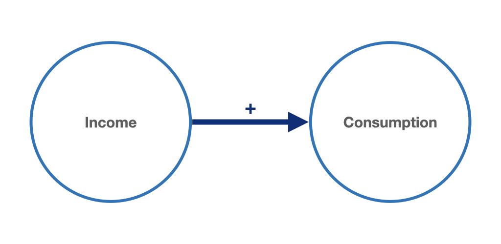
Figure 3.2: The absolute income hypothesis: current aggregate income as an important determinant of aggregate consumption.
We can use the absolute income hypothesis to construct an initial formal behavioural equation for our macroeconomic model. For the behavioural equation of aggregate consumption, we assume in the simplest case that total disposable income, \(Y_d\), of households is identical to total income, \(Y\), of our economy (\(Y_d = Y\)). Thus, we are making the simplifying assumption that all income is paid to households in the form of wages and profits and that no taxes are paid to the government. The behavioural equation of total consumption, \(C\), according to the absolute income hypothesis can then be represented as a linear function of total income:
\[\begin{equation} C = C(Y) = c_a + c_Y Y \tag{3.1} \end{equation}\]
Equation (3.1) is referred to as the Keynesian consumption function. It is assumed that total consumption is composed of a non-income-dependent part and an income-dependent part. The income-independent part is given by the first term of the consumption function, \(c_a\), and is called autonomous consumption. The autonomous part of the consumption function gives the level of consumption that would result if households had no income at all. It is thus a kind of “minimum consumption” that households want to maintain or even have to maintain for subsistence reasons. In contrast, the level of the income-dependent part of the consumption function, \(c_Y Y\), depends on current disposable income, \(Y\). Here, the parameter \(c_Y\) determines how large the increase in consumption is when income increases. Hence, \(c_Y\) is referred to as the marginal propensity to consume. Since the absolute income hypothesis postulates that consumption increases less than income, the marginal propensity to consume in the Keynesian consumption function takes a value between zero and one (\(0 < c_Y < 1\)). For example, a marginal propensity to consume of \(0.6\) would mean that an increase in income of 100 euros would increase private consumption by 60 euros. The marginal propensity to consume, \(MPC\), in the equation (3.1), therefore gives the slope of the consumption function:15
\[\begin{equation} MPC ≡ \frac{\Delta C}{\Delta Y} = c_Y \tag{3.2} \end{equation}\]
We can also graph the consumption function. For autonomous consumption, we choose \(c_a = 30\) and for the marginal propensity to consume we choose \(c_Y = 0.5\). Our consumption function then becomes:
\[\begin{equation} C = \underbrace{30}_{\text{autonomous consumption}} + \underbrace{0.5 \cdot Y}_{\text{consumption dependent on income}} \tag{3.3} \end{equation}\]
This numerical example of the Keynesian consumption function is shown in figure 3.3:
Figure 3.3: Keynesian consumption function.
3.2 Taxes in the consumption function
When the government collects taxes and makes transfers to households, aggregate disposable income of households, \(Y_d\), is generally not the same as aggregate income, \(Y\). This is what would happen unless we assume that the government transfers to households as much as it has previously collected in taxes, for example by taxing rich households and firms and transferring those revenues as social benefits to poorer households.
However, if net taxation, i.e. the difference between taxes and transfers, is positive, so that the government can finance its spending on goods and services, this would have, at least initially, a negative impact on households’ total disposable income. It should be noted, however, that we do not yet consider the effect that government spending financed by tax revenues might have on disposable income.16
With the introduction of taxes in our Keynesian consumption function, households consumption now depends on disposable income:17
\[\begin{equation} C = c_a + c_{Y_d} Y_d \tag{3.4} \end{equation}\]
A positive net taxation of private consumption would initially have a negative impact on consumption demand. Figure 3.4 illustrates the causal relationships between taxation and disposable income of the household sector and between disposable income and consumption.
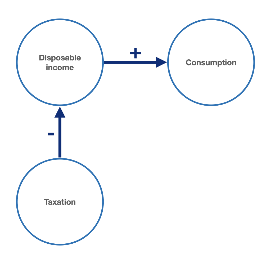
Figure 3.4: Absolute income hypothesis with taxes: causal relationship between taxation, disposable income and consumption.
To illustrate these relationships within the Keynesian consumption function (3.4), assume for the simplest case that total net tax revenue, \(T\), net of government transfers, is given by a lump sum independent of income:
\[\begin{equation} T = \overline{T} \tag{3.5} \end{equation}\]
The disposable income of the household sector thus becomes:
\[\begin{equation} Y_d = Y - T \tag{3.6} \end{equation}\]
By substituting (3.6) in (3.4), our consumption function becomes:
\[\begin{equation} C = c_a + c_{Y_d} (Y - T) \tag{3.7} \end{equation}\]
In (3.7), we have labeled the \(MPC\) from disposable income as \(c_{Y_d}\).
Since, compared to the consumption function without taxes from (3.1), the constant has changed from \(c_a\) to \(c_a - c_{Y_d} T\) in (3.7), the consumption function with lump-sum taxation shifted downward in parallel with respect to the consumption function without taxation of figure 3.3, as figure 3.5 shows:
Figure 3.5: Keynesian consumption function with and without income-independent lump-sum taxation.
Given that a change in aggregate income, \(Y\), with no change in taxation, \(T = \overline{T}\), entails a change in disposable income of the same amount, under non-income taxation, the \(MPC\) from aggregate income, \(c_Y = \frac{\Delta C}{\Delta Y}\), and the \(MPC\) from disposable income, \(c_{Y_d} = \frac{\Delta C}{\Delta Y_d}\), are equal: \(c_Y = c_{Y_d}\).
Disposable income is again the difference between total income and net tax revenues: \(Y_d = Y - T = Y - tY = (1 - t) Y\). The Keynesian consumption function changes accordingly. We substitute \(Y_d\) into (3.4) and obtain:
\[\begin{equation} T = tY \tag{3.8} \end{equation}\]
For the average net tax rate, \(t\), the following applies: \(0 < t < 1\).
Disposable income is again the difference between total income and net tax revenues: \(Y_d = Y - T = Y - tY = (1 - t) Y\). The Keynesian consumption function changes accordingly to by substituting \(Y_d\) into (3.4):
\[\begin{equation} C = c_a + c_{Y_d} (1 - t)Y \tag{3.9} \end{equation}\]
The \(MPC\) with respect to a change in disposable income is now:
\[\begin{equation} \frac{\Delta C}{\Delta Y_d} = c_{Y_d} \tag{3.10} \end{equation}\]
In contrast, the marginal propensity to consume with respect to a change in total income, \(Y\), in equation (3.9) now holds:
\[\begin{equation} \frac{\Delta C}{\Delta Y} = c_{Y_d} (1 - t) \tag{3.11} \end{equation}\]
Figure 3.6 shows the consumption function as a function of aggregate income, \(Y\), once with taxes and transfers (equation (3.9)) and once without (equation (3.1)) taxes and transfers. Continuing to assume the same numerical values as in the previous numerical example of our consumption function and assuming a value for the average net tax rate of \(t = 0.2\), we have:
\[C = \underbrace{30}_{\text{autonomous consumption}} + \quad \underbrace{0.5\quad \cdot \underbrace{(1-0.2) \cdot Y}_{\text{disposable income}}}_{\text{consumption dependent on income}} = \quad 30 \quad + \quad 0.4 \cdot Y\]
Here, the introduction of taxes and transfers reduces the increase in the consumption function with respect to total income, \(\frac{\Delta C}{\Delta Y} = c_{Y_d} (1 - t)\), since disposable income is reduced by net tax revenue, \(tY\), compared to the consumption function without taxes (3.1). In figure 3.6, the consumption function with taxes and transfers dependent on income is less steep with respect to the consumption function with no taxes.
Figure 3.6: Keynesian consumption function with and without taxation dependent on income.
In the interactive app accessible through the link below, the parameters of the consumption function in (3.9) can be freely defined. Setting the average net tax rate, \(t\), to zero yields the simple Keynesian consumption function without taxes and transfers.
3.3 The saving function of private households
Households can decide to use their income for consumption purposes or they may decide to save it. This implies that a consumption function, \(C\), has always a counterpart, the saving function, \(S\). As with consumption, saving is also a flow variable.
The saving function is defined as the difference between households’ income, here excluding taxes, i.e. \(Y = Y_d\), and their consumption expenditure, \(C\):
\[\begin{equation} S = Y - C \tag{3.12} \end{equation}\]
Assuming the simple Keynesian consumption function without taxes from (3.1), we have:
\[\begin{equation} S = Y - (c_a + c_Y Y) \tag{3.13} \end{equation}\]
therefore:
\[S = Y - c_a - c_Y Y\]
or:
\[\begin{equation} S = - c_a + (1 - c_Y) Y \tag{3.14} \end{equation}\]
Figure 3.7 graphically represents equation (3.14) where \((1 - c_Y)\) is the marginal propensity to save, or \(MPS\) for short.
Figure 3.7: The saving function.
Further reading on chapter 3
Textbooks:
- Hein (2023, chaps. 3–4)
- Carlin and Soskice (2015, chap. 1.2)
- Froyen (2002, chap. 5)
- Bofinger (2019, chap. 17.4) (in German)
- Heine and Herr (2013, chap. 4.4) (in German)
Other literature:
- Keynes (1936, chaps. 8–10)
Literature
The slope of a function is given by its first derivative. The first derivative, \(\frac{\Delta y}{\Delta x}\) or \(\frac{dy}{dx}\), of a linear function of the form \(y = mx + b\) is \(\frac{\Delta y}{\Delta x} = m\). Thus, the value \(m\) is the slope. For an explanation of the slope and the derivative rules, see appendix B.↩︎
See section 6.2.↩︎
The subscript \(_d\) stands for “disposable”.↩︎